Solving a TRUST problem requires the user to select a certain discretization which allows the code to pass the treated equations from a continuous to a discretized form.

TRUST supports mainly four discretizations, all derived from the C++ class Discretisation_base. Click here to see the Doxygen documentation of this class.

The choice of the discretization is dependent on the mesh type and (can be, not always …) on the problem. Here are the available discretizations in the TRUST platform.

The Finite Volume Difference (VDF) discretization

The VDF discretization (class VDF_discretisation and alias VDF) is the simplest and the most performant discretization of the TRUST plaform. This discretization is compatible with conform mesh with hexahedral type of elements. Attention: do not confuse between a hexahedral mesh and a cartesian mesh. The VDF mesh is not structured and does not follow the IJK indexing !

As stated by its name, the VDF is a conservative finite volume scheme of Marker-and-Cell (MAC) type. The discretization of each term of the equation is performed by integrating over a control volume. The diffusion gradient terms are approximated by a linear difference equation. All scalars are stored at the center of each control volume except the velocity field which is defined on a staggered mesh.

This discretization supports 2D axi-symetrical configurations and is compatible with Pb_Multiphase.

2D staggered grid zoomed VDF description: scalars stored at the cell center (black points), x−horizontal velocity component at the horizontal faces of the cell (green point), y−horizontal velocity component at the vertical faces of the cell (red point). Green and red dotted control volumes are used to solve the horizontal (green) and vertical (red) velocity components equations.

The Finite Element Volume (VEF) discretization

The VEF discretization (classes VEF_discretisation and alias VEFPreP1B) is used when the mesh is conform but with tetrahedral elements (triangles in 2D). This numerical scheme combines finite volume and finite elements to integrate in conservative form all conservation equations over the control volumes belonging to the calculation domain.

As in the classical Crouzeix–Raviart element, both vector and scalar quantities are located at the centers of the faces. The pressure, however, is located at the vertices and at the center of gravity of a tetrahedral element (in 3D, triangles in 2D).

This discretization leads to very good pressure/velocity coupling and has a very dense divergence free basis. Along this staggered mesh arrangement, the unknowns, i.e. the vector and scalar values, are expressed using non-conforming linear shape-functions (P1-nonconforming). The shape function for the pressure is constant for the center of the element (P0) and linear for the vertices (P1).

This discretization does not support 2D axi-symetrical configurations and is not compatible with Pb_Multiphase.

2D zoomed VEF description: scalars (except pressure) and velocity vector field are stored at the centers of the faces (red arrows). Pressure at the center of each triangle and at the vertices (black points).

The PolyMAC-series discretization

The PolyMAC discretization is a series of Marker-and-Cell (MAC) schemes that can handle any type of mesh (non-conform, non-orthogonal, poly-hedral types, …). The numerical description of this schemes is quite complex and depends on the employed version. Here is a summary of the PolyMAC versions available in the TRUST platform. This discretization (with all versions) does not support 2D axi-symetrical configurations but is compatible with Pb_Multiphase (in fact it was the first discretization for which Multiphase Problem was available).

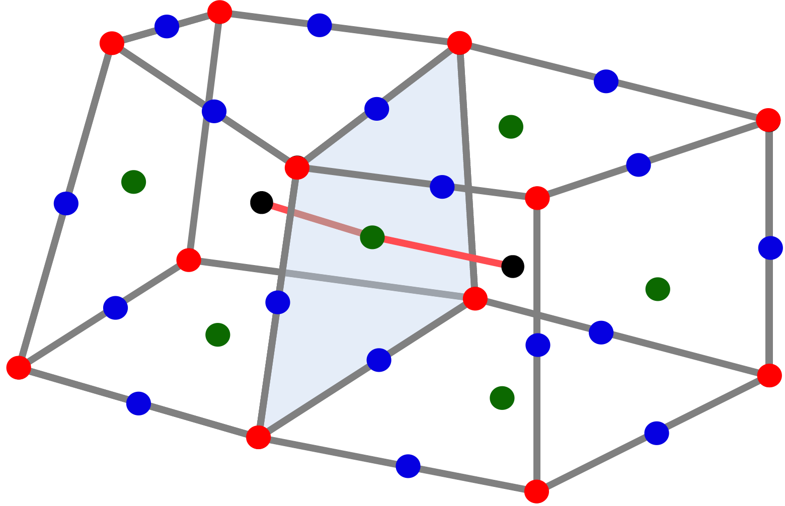3D illustration of the storing locations used with the PolyMAC discretization.
Elements at black points, faces at green points, nodes at red points and edges at blue points.

• PolyMAC_P0P1NC

  This is the first PolyMAC version introduced in the TRUST platform. The corresponding C++ class is simply PolyMAC_discretisation (the aliases are PolyMAC_P0P1nc, or simply PolyMAC). In this version, the scalars (except the pressure and temperature) are stored at the center of the elements (black points) whatever the type of the element is.

  At the faces of each element (green points), the scalar product of the velocity and the face normal are stored (as in VDF if the mesh is hexahedral). Additional auxiliary variables stored at the edges of each cell (blue points) are used. They correspond to the scalar product of the vorticity field and the vector tangent to each edge.

  The main pressure and temperature fields are stored at the elements (black points). Additional auxiliary variables are used for both fields and the values are stored at the faces (green points). These auxiliary variables are completely treated as unknowns and they contribute in the matrix construction.

• PolyMAC_P0

  The corresponding C++ class is simply PolyMAC_P0_discretisation (the alias is PolyMAC_P0). In this version, scalars quatities are stored at the center of the elements (black points) whatever the type of the element is.

  At the faces of each element (green points), the scalar product of the velocity and the face normal are stored (as in VDF if the mesh is hexahedral). Additional auxiliary variables correstponding to the complete velocity vector field are used. They are stored at the center of each cell (black points) and contribute in the matrix construction.

• PolyMAC_P1

  The corresponding C++ class is simply PolyMAC_P1_discretisation (the alias is PolyMAC_P1). In this version, the scalars (except the pressure and temperature) are stored at the center of the elements, in addition the complete velocity vector field (black points). The pressure and temperature unknowns are stored at the nodes (red points).

• PolyVEF

  The corresponding C++ class is simply PolyVEF_discretisation (the alias is PolyVEF). In this version, the scalars (except the pressure and temperature) are stored at the center of the elements (black points). The velocity vector field is stoced at the faces of each element (green points). The pressure and temperature unknowns are stored at the center of the elements and at the nodes (black and red points).

Mesh stencil illustrated with the PolyMAC discretization.

Examples of computational domains/meshes used with the PolyMAC discretization.

The Finite Element (EF) discretization

The EF discretization (class EF_discretisation) implements a classical finite element method. This discretization supports 1D mesh types. This discretization supports 2D axi-symetrical configuration, but is not compatible with Pb_Multiphase.