Turbulent Flow with Concentration

This tutorial demonstrates how to simulate a 2D incompressible turbulent flow with constituent transport using TrioCFD’s k-ε model. Figure 6 shows the geometry of the test case you will run in this tutorial.

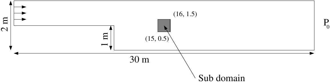
Figure 6 Geometry of the downward march case

Problem Setup

Fluid Properties

Property	Value
Dynamic viscosity \(μ\)	\(3.7 \cdot 10^{-5} kg \cdot m^{-1} \cdot s^{-1}\)
Density \(ρ\)	\(2 kg \cdot m^{-3}\)
Reynolds number \(Re\)	54,054

Boundary Conditions

Location	Velocity	Pressure	k	ε	Notes
Inlet	\(U_0 = 1 m \cdot s^{-1}\)	-	\(10^{-2}\)	\(10^{-3}\)	Imposed velocity, dimensionless k and ε
Outlet	-	\(P_0 = 0\)	0	0	Constant pressure
Top/Bottom walls	\(U = 0\)	-	Standard flux	Null	No-slip condition

Study Template Preparation

To start, copy the base Marche study, which provides a foundation for 2D incompressible turbulent flow using the k-ε model.

Navigate to your working directory: $MY_TRUST_TUTORIAL and execute:

triocfd -copy Marche

Since we’ll be working with constituent diffusion, the Constituants study also needs to be copied as it demonstrates 2D incompressible laminar flow with constituents:

triocfd -copy Constituants

Documentation access is available through the TrioCFD index system, which provides access to the Reference Manual containing the necessary keywords for problem configuration:

triocfd -index

You can also find those informations in the TrioCFD Documentation

Test Case Implementation

Problem Configuration and Constituent Setup

First, open the Marche.data file.

The data file modification begins by renaming the problem to accommodate concentration equations.

Check the TrioCFD Reference Manual to find the appropriate keywords.

Then, add 3 constituents of equal diffusivities (\(\alpha = 1 m \cdot s ^{-1}\)) in the block problem after the fluid definition)

Define the concentration equation into the problem with the correct initial (\(C_1 = C_2 = C_3 = 0\)) and boundary conditions. Remember that concentrations are a vectors of 3 components.

Use the Schmidt model to close the turbulence model in the concentration equation

Turbulence Model Modification

Chage the Navier-Stokes turbulence model to an anisotropic concentration-coupled version: Source_Transport_K_Eps_aniso_concen { C1_eps 1.44 C2_eps 1.92 C3_eps 1. }

This modification ensures proper coupling between the flow field and concentration transport.

Additionally, the fluid definition must include a volume expansion coefficient for concentration (beta_co) set as a uniform field equal to 0, along with a gravity field initialized to 0.

Initial Validation and Sub-domain Definition

Try to run your update test case:

triocfd marche

Now, you will define the sub domain in grey in Figure 6.

To do so, you will need to use the Sous_Zone keyword. To find an example of the Sous_Zone keyword usage, run the following:

trust -search Sous_Zone

It will give you tha list of TRUST test cases that use this keyword. You can for example edit the PCR.data file of the PCR test case.

Source Term Implementation

The second constituent requires a specific source term (S₂ = 1 m⁻³) applied exclusively to the defined sub-domain. This implementation uses the Champ_Uniforme_Morceaux keyword to ensure spatial localization of the source effects.

Post-processing and run

Now, add a source term for the second constituent only ($S_2 = 1 m^{-3}) applied on the sub domain thanks to the keyword Champ_Uniforme_Morceaux.

Change post-processing format to lata in the post-processing block.

Add the keywords concentration0, concentration1, concentration2 in the fields of the post-processing block to write the 3 concentrations into the .lata file.

Run the calculation:

triocfd marche

And check the results with Visit. You will be able to see the different concentrations.