Tank filling (3D)

Description of the setup

Figure 10 shows the geometry of the test case you will run in this tutorial. It consists of a 3D tank initially half-filled with liquid, a front-tracking interface separating liquid and gas. There is a rotating solid in the liquid and a droplet in the gas above the liquid. The problem will be treated with a 3D structured mesh (VDF discretisation of TRUST).

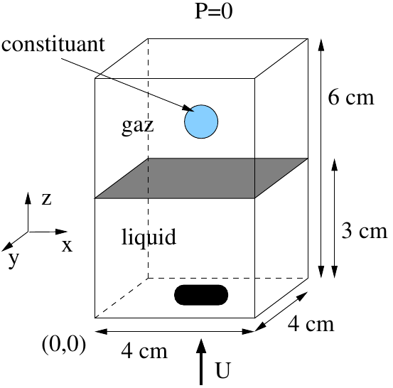
Figure 10 Geometry of the tank

Fluid Properties

Phase	Property	Value
Liquid	\(\rho\)	\(1000 kg.m^{-3}\)
Liquid	\(\mu\)	\(2.82 \times 10^{-4} kg.m^{-1}.s^{-1}\)
Liquid	\(\sigma\)	\(0.05 N.m^{-1}\)
Liquid	\(D\)	\(10^{-6} m^2.s^{-1}\)
Gas	\(\rho\)	\(100 kg.m^{-3}\)
Gas	\(\mu\)	\(2.82 \times 10^{-4} kg.m^{-1}.s^{-1}\)

Boundary Conditions

Location	Condition
Up	Free outlet
Down	\(V=(0,0,10^{-3} m/s)\)
Walls	\(V=0\)

Initial Conditions

\(V=0\)

\(C=e^{(-((x-0.02)^{2}+(y-0.02)^{2}+(z-0.03)^{2})/0.03^{2})}\)

The initial interface between the air and the gas is a parabolic function.

Tutorial setup

First, go to an empty directory and copy the base TrioCFD test case from which we will start: FTD_all_VDF

triocfd -copy FTD_all_VDF && cd FTD_all_VDF

Open the datafile FTD_all_VDF.data in a text editor of your choice.

A few remarks:

• The Front-tracking module of TrioCFD is not extensively tested in 2D. It may not be reliable.

• The use of the front tracking module is indicated by the type of problem: Probleme_FT_Disc_gen is used here

• In the Navier-Stokes equation of Probleme_FT_Disc_gen, the use of the keyword modele_turbulence is mandatory. For a laminar problem, specify modele_turbulence nul.

Modifying the test case

Start by making some changes in the file FTD_all_VDF.data:

• Increase the height of the tank from 0.06 to 0.12

  • Do not forget to adapt boundary definitions

• Increase the max time tmax in Scheme_euler_explicit to 0.5 (or more)

• Add a second droplet above the first one, at z=0.08.

  • keyword ajout_phase0 could be useful. Look in the Keyword Reference Manual for ajout_phase0/ajout_phase1

  • It is also possible to access the reference manual with triocfd -index

  • Do not forget commas between the two definition of each droplet

• Change the postprocessing period dt_post of each postprocessing block from 0.05 to 0.01

  • in the first one, add format lata

• The first postprocessing block (Post_processing) is the classical block for post-processing probes and fields. Here, we want to see the concentration field and the indicatrice_interf field. Value of this field is 0 for liquid and 1 for gas, so the interface is located at indicatrice value 0.5

• Change the interpolation location of indicatrice_interf and the concentration fields in the first post-processing block, by adding the keyword elem just after the fields.

  • the values in the post-processing tool will be plotted at the center of each element of the mesh.

  • this is done in the block right before liste_postraitements.

• The second postprocessing block (postraitement_ft_lata in liste_postraitements) allows to visualize the moving mesh of the interface. It can be visualized with visit.

• For each interface, several fields can be obtained:

  • curvature, with the courbure keyword

  • velocity interface, with the vitesse keyword

  • pe, used here, is for debugging purposes

  • locations can be som for mesh nodes or elem for mesh cells

Running and visualizing the simulation

Now, you can run the calculation:

triocfd FTD_all_VDF

You can follow the time step evolution by having a look at the FTD_all_VDF.dt_ev file. It contains on each line the physical time, the time step, security factor and residuals.

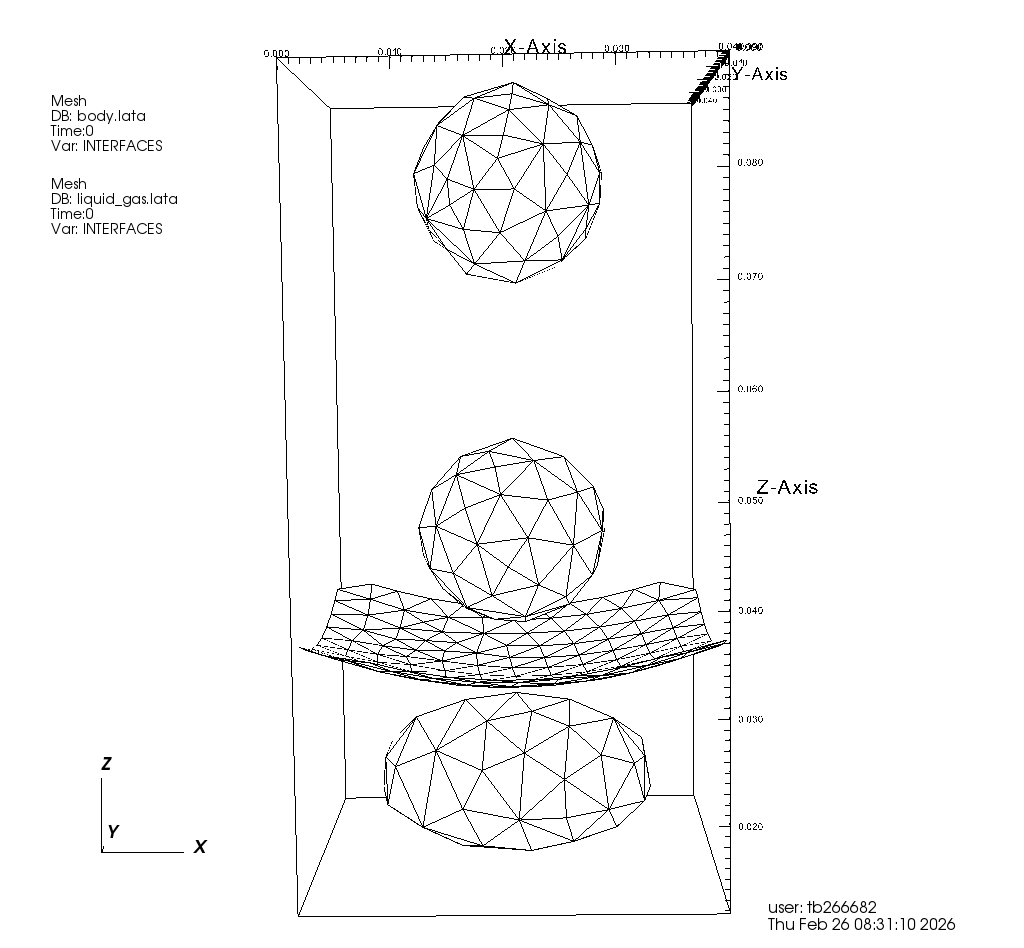
Using visit, visualize the interface and the concentration field. For that, you have to open the lata from the liste_postraitements block: body.lata and liquid_gas.lata. See below for detailed instructions:

Open visit, then in visit:

• Click Open, set filter to *lata and select body.lata

• set body.lata as active source

  • In Plots, click add, then Mesh and finally INTERFACES

  • Click Draw

• Click Open and select liquid_gas.lata

• set liquid_gas.lata as active source

  • In Plots, click add, then Mesh and finally INTERFACES

  • In popup window Correlate databases, select Yes. If the popup does not show, close visit and restart from beginning. Or add the correlation manually if you know how to.

  • Click Draw

• Using the Time Slider Correlation1, you should be able to see the droplets fall, the solid rotate and the surface oscillate.

Click to display expected result

Now try visualizing the concentration field.