
Turbulent Flow over a backward-facing step (3D)#
Description of the case#
Figure 9 shows the geometry of the test case you will run in this tutorial.
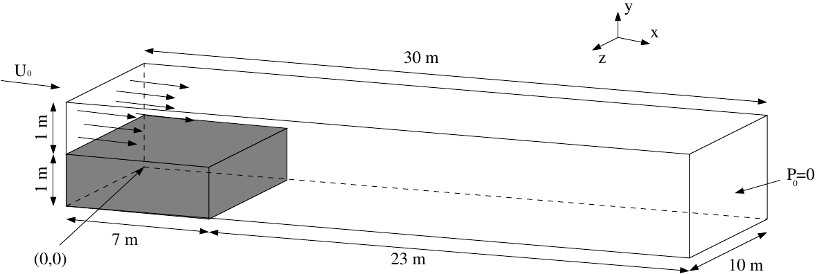
Figure 9 Geometry of the step#
Fluid Properties#
Property |
Value |
|---|---|
\(\rho\) |
\(2 kg.m^{-3}\) |
\(\mu\) |
\(5.10^{-5} kg.m^{-1}.s^{-1}\) |
Boundary Conditions#
Location |
Condition |
|---|---|
Inlet |
\(U_0=1 m.s^{-1}\) |
Outlet |
\(P_0=0\) |
with \(Re=\frac{U_0 H_{inlet} \rho}{\mu} = \frac{1 \times 1 \times 2}{5.10^{-5}} = 40000\)
Tutorial setup#
First, go to an empty directory and copy the base TrioCFD test case from which we will start: Marche3D
triocfd -copy Marche3D && cd Marche3D
Open the datafile Marche3D.data in a text editor of your choice.
Notice that we use a Pb_Hydraulique_Turbulent problem with Navier_Stokes_Turbulent equation, which has a modele_turbulence keyword for the turbulence.
Modifying the test case#
Start by making some changes in the file Marche3D.data:
Modify the fluid characteristics for a calculation at Reynolds number \(Re = 50000\):
this is done in the block
fluide_incompressible.For exemple, use \(\rho = 1 kg.m^{-3}\) and \(\mu = 2.10^{-5} kg.m^{-1}.s^{-1}\).
Change the turbulence model for a subgrid Smagorinsky model with standard wall law:
replace
sous_maillebysous_maille_smago.Look into Keyword Reference Manual to find the keywords and the parameters that you can tweak.
Change the convection scheme to
quick. This happends in the blockconvectionof the equation.amontis currently used.In the
Post_processingblock, addformat latato ease visualization with visit.Postprocess the fields velocity, pressure, vorticity and turbulent viscosity at the nodes (
som) and elements (elem).only vorticity should be missing
Running and visualizing the simulation#
Now, you can run the calculation:
triocfd Marche3D
Have a look at the postprocessed fields using visit.
Using a RANS turbulence model#
This next part of the tutorial will guide you toward using a RANS turbulence model with TrioCFD, starting from the previous LES simulation. This is fairly hard to do by yourself. The detailed instructions should cover everything, but the complete solution is below hidden in a dropdown menu.
Edit the file Marche3D.data again, to change the turbulence model for a RANS k-epsilon model.
You need to replace
sous_maille_smagobyk_epsilon.In the
k_epsilonblock, you will need to add several keywords:The
transport_equationkeyword is mandatory. You must specifytransport_equation transport_k_epsilon { ... }Inside the
transport_k_epsilonblock, you must specify theconvectionanddiffusionschemes (see bloc_convection and bloc_diffusion)Then, you also need to define the
boundary_conditions:For that, you can copy the ones from
Navier_Stokes_Turbulentabove and do some slight adaptations.Replace
Paroi_Fixewithparoito use the wall law.In the 2
SortieXXXboundaries, replacefrontiere_ouverte_pression_imposeewithfrontiere_ouverte k_eps_ext. This boundary conditions expects a field with two components (for k and eps). ReplaceChamp_Front_Uniforme 1 0.withChamp_Front_Uniforme 2 0. 0.. It is used on this equation to let k and eps leave through the boundary, but in case of reentering flow, force the entering values of k and eps.For the
Entree, usefrontiere_ouverte_k_eps_impose, which takes a field with 2 components again, and choose pertinent values of k and eps (not 0 or nothing will happen).
Finally, you need to specify
initial_conditions. You can also copy the one fromNavier_Stokes_Turbulentabove. Here, you need to initialize the fieldk_Eps(probably with the same values as in theEntreeboundary).
Now, you can run the test case again and visualize the results.
SPOILER: solution for the RANS model
modele_turbulence k_epsilon {
    transport_equation transport_k_epsilon {
            convection { amont }
            diffusion { }

            boundary_conditions
            {
                Bas1 paroi
                Haut1 paroi
                Haut2 paroi
                Haut3 paroi
                Bas2 paroi
                Gauche paroi
                Bas3 paroi
                Sud1 paroi
                Nord1 paroi
                Sud2 paroi
                Nord2 paroi
                Sud3 paroi
                Nord3 paroi
                Sud4 paroi
                Nord4 paroi
                Sud5 paroi
                Nord5 paroi
                SortieBasse frontiere_ouverte k_eps_ext Champ_Front_Uniforme 2 0. 0.
                SortieHaute frontiere_ouverte k_eps_ext Champ_Front_Uniforme 2 0. 0.
                Entree frontiere_ouverte_k_eps_impose Champ_Front_Uniforme 2  0.405 7.73
            }

            initial_conditions
            {
                k_Eps Champ_Uniforme 2 0.405 7.73 # taken from another test case, may not be pertinent #
            }
    }
    TURBULENCE_PAROI loi_standard_hydr
}