
Thermal modeling#
There are 3 types of thermal fluxes available in TrioCFD multiphase:
The interfacial heat flux \(h_k(\alpha,T,P)\)
The wall heat flux \(q_{pk}(\alpha,T,P)\)
The phase change flux \(G(\alpha,T,P)\)
The computation of condensation and evaporation is done in Source_Flux_interfacial_base:
void Source_Flux_interfacial_base::set_param(Param& param)
{
  const Pb_Multiphase& pbm = ref_cast(Pb_Multiphase, equation().probleme());
  if (!pbm.has_correlation("flux_interfacial"))
    Process::exit(que_suis_je() + ": a flux_interfacial correlation must be defined in the global correlations { } block!");

  correlation_ = pbm.get_correlation("flux_interfacial");

  dv_min = ref_cast(Flux_interfacial_base, correlation_->valeur()).dv_min();

  return is;
}
with \(\texttt{n_lim}=\begin{cases} -1,\ \text{if G won't make the phase evanescent}\\ \text{number of the evanescent phase, otherwise.} \end{cases}\)
If saturation activated then:
If no correlation for G or if \(|\frac{\Phi}{L}|<|G|\) (limitation by energy conservation) then:
The phase change G is limited by evanescence at \(G_{\text{lim}}\) (see evanescence part).
If there is no evanescence and no phase change model then:
These fluxes are then distributed to the following equations:
Mass equation as source/sink
Energy equation as heat transfer
Interfacial area concentration as condensation/nucleation (cf equivalent diameter section)
The model is implemented as follows:
In the energy equation:
If saturation is activated, then in the mass equation we get:
if there is no evanescence then:
If saturation is activated, then in the energy equation we get:
with \(c\) the minority phase side to respect the energy conservation in case of evanescence.
Interfacial heat flux#
The general expression of the interfacial heat flux is:
The model is implemented in:
void Flux_interfacial_base::set_param(Param& param)
The available input parameters are:
    double dh;            // Hydraulic diameter
    const double *alpha;  // Void fraction
    const double *T;      // Temperature
    const double *T_passe;// Previous time temperature
    double p;             // Pressure
    const double *nv;     // Norme of relative velocity
    const double *lambda; // Thermal conductivity
    const double *mu;     // Viscosity
    const double *rho;    // Density
    const double *Cp;     // Calorific capacity
    const double *Lvap;   // Latent heat
    const double *dP_Lvap;// Phase change latent heat
    const double *h;      // Enthalpy
    const double *dP_h;   // Enthalpy derivative regarding pressure
    const double *dT_h;   // Enthalpy derivative regarding temperature
    const double *d_bulles;//Bubble diameter
    const double *k_turb; // Turbulent kinetic energy
    const double *nut;    // Turbulent viscosity
    const double *sigma;  // Superficial tension
    DoubleTab v;          // Velocity
    int e;                // Element index
The interfacial heat flux operator must fill hi tab so that:
\(\texttt{hi}({\color{myteal}k1}, {\color{mydarkorchid}k2})\) and \(\texttt{hi}({\color{mydarkorchid}k2},{\color{myteal}k1})\) exchange coefficients
\(\texttt{dT_hi}({\color{myteal}k1}, {\color{mydarkorchid}k2},n)\) and \(\texttt{dT_hi}({\color{mydarkorchid}k2},{\color{myteal}k1},n)\) Exchange coefficient derivative regarding the temperature
\(\texttt{da_hi}({\color{myteal}k1}, {\color{mydarkorchid}k2}, n)\) and \(\texttt{da_hi}({\color{mydarkorchid}k2}, {\color{myteal}k1}, n)\) Exchange coefficient derivative regarding void fraction of phase n
\(\texttt{dp_hi}({\color{myteal}k1}, {\color{mydarkorchid}k2})\) and \(\texttt{dp_hi}({\color{mydarkorchid}k2}, {\color{myteal}k1})\) Exchange coefficient derivative regarding pressure
Availability of drift models in TrioCFD/CMFD.
Model |
Used |
Validated |
Test case |
|---|---|---|---|
Constant |
Yes |
Yes |
TrioCFD/CoolProp, TrioCFD/Gabillet, TrioCFD/Canal axi two-phase, Trust/Canal bouillant two-phase, Trust/Canal bouillant drift, Trust/Comparaison lois eau |
Chen-Mayinger |
Yes |
No |
|
Kim-Park |
Yes |
No |
|
Ranz-Marshall |
Yes |
No |
|
Wolfert |
Yes |
No |
|
Wolfert compsant |
Yes |
No |
|
Zeitoun |
Yes |
No |
Constant#
The model is implemented in:
void Flux_interfacial_Coef_Constant::set_param(Param& param)
{
param.ajouter(pbm.nom_phase(n), &h_phase(n), Param::REQUIRED);
}
Default values: ?
The model implemented is:
Chen and Mayinger#
The model is implemented in:
void Flux_interfacial_Chen_Mayinger::set_param(Param& param)
Default values: ?
The model implemented is:
with
\(Re_b=\frac{\rho_l d_b (u_g-u_l)}{\mu_l}\)
\(Pr\frac{\mu_l Cp_l}{\lambda_l}\)
Kim and park#
The model is also described in REFNEC and is implemented in:
void Flux_interfacial_Kim_Park::set_param(Param& param)
Default values: ?
The model implemented is:
with
\(Re_b=\frac{\rho_l d_b (u_g-u_l)}{\mu_l}\)
\(Pr\frac{\mu_l Cp_l}{\lambda_l}\)
\(Ja=\frac{\rho_lCp_l(T_g-T_l)}{\rho_gL_{vap}}\)
Ranz Marshall#
The model is also described in REFNEC and is implemented in:
void Flux_interfacial_Ranz_Marshall::set_param(Param& param)
{
param.ajouter("dv_min", &dv_min_);
}
Default values:
\(\texttt{a_min}= 0.01\).
The model implemented is:
with
\(Re_b=\frac{\rho_l d (u_g-u_l)}{\mu_l}\)
\(Pr = \frac{\mu_l Cp_l}{\lambda_l}\)
Wolfert#
The model is also described in REFNEC and is implemented in:
void Flux_interfacial_Wolfert::set_param(Param& param)
{
param.ajouter("Pr_t", &Pr_t_);
}
Default values:
\(\texttt{Pr_t_} = 0.85\).
The model implemented is:
with
\(Ja=\frac{\rho_l Cp_l (T_g-T_l)}{\rho_lLvap}\)
\(Pe\frac{\rho_l Cp_l (u_g-u_l)d}{\lambda_l}\)
\texttt{M_PI} = \(\pi\)
Wolfert compsant (To be erased)#
The model is also described in REFNEC and is implemented in:
void Flux_interfacial_Wolfert_composant::set_param(Param& param)
{
  param.ajouter("Pr_t", &Pr_t_);
  param.ajouter("dv_min", &dv_min_);
}
Default values:
\(\texttt{Pr_t_ = 0.85}\).
The model implemented is:
with
\(Ja=\frac{\rho_l Cp_l (T_g-T_l)}{\rho_lLvap}\)
\(Pe=\frac{\rho_l Cp_l (u_g-u_l)d}{\lambda_l}\)
\(U_\tau = 0.1987 (u_g-u_l) (\frac{D_h\rho_l (u_g-u_l)}{\mu_l})^{-1/8}\)
\(\lambda_t = 0.06Pr_t U_\tau D_h \)
\texttt{M_PI} = \(\pi\)
Zeitoun#
The model is also described in REFNEC and is implemented in:
void Flux_interfacial_Zeitoun::set_param(Param& param)
{
param.ajouter("dv_min", &dv_min_);
  if (a_res_ < 1.e-12)
    {
      a_res_ = ref_cast(QDM_Multiphase, pb_->equation(0)).alpha_res();
      a_res_ = std::max(1.e-4, a_res_*10.);
    }
}
Default values:
\(\texttt{a_min_coeff} = 0.1\),
\(\texttt{a_min} = 0.01\),
\(\texttt{a_res_} = -1.\)
The model implemented is:
If \(( T_g > T_l)\) then:
And if \(\alpha_g < \text{a_res_}\) then:
End. Else (Temperature condition)
with
\(Re_b = \frac{\rho_l (u_g-u_l)d_b}{\mu_l}\)
\(Ja=\frac{max(T_g-T_l,2.)\rho_l Cp_l}{\rho_lLvap}\)
\(dP_{Ja}=\frac{max(T_g-T_l,2.)\rho_l Cp_l}{\rho_l}\frac{-dP_{vap}}{Lvap^2}\)
\(dT_{gJa}=\begin{cases}\frac{\rho_lCp_l}{\rho_gLvap},\ if\ T_g-T_l> 2.\\ 0,\text{ otherwise} \end{cases}\)
\(dT_{lJa}=\begin{cases}\frac{-\rho_lCp_l}{\rho_gLvap},\ if\ T_g-T_l> 2.\\ 0,\text{ otherwise}\end{cases}\)
\(da_{Nu} = 2.04 Re_b^{0.61}Ja^{-1.308}\begin{cases} 0.328(\alpha_g^{0.328-1},\text{ if }\alpha_g > \texttt{a_min_coeff}\\ 0,\text{ otherwise} \end{cases}\)
\(dP_{Nu} = 2.04Re_b^{0.61} \max(\alpha_g, \texttt{a_min_coeff})^{0.328} -0.308dP_{Ja} Ja^{-1.308}\)
\(dT_{gNu} = 2.04Re_b^{0.61} \max(\alpha_g, \texttt{a_min_coeff})^{0.328} -0.308dT_{Ja} Ja^{-1.308}\)
\(dT_{lNu} = 2.04Re_b^{0.61} \max(\alpha_g, \texttt{a_min_coeff})^{0.328} -0.308dT_{Ja} Ja^{-1.308}\)
Wall heat flux#
The general expression of the wall heat flux is:
The model is implemented in:
void Flux_parietal_base::set_param(Param& param)
The available input parameters are:
    int N;                // Number of phases
    int f;                // face number
    double y;             // distance between the face and the center of gravity of the cell
    double D_h;           // Hydraulic diameter
    double D_ch;          // Heated hydraulic  diameter
    double p;             // Pressure
    double Tp;            // Wall temperature
    const double *alpha;  // Void fraction
    const double *T;      // Temperature
    const double *v;      // Velocity norm
    const double *lambda; // Thermal conductivity
    const double *mu;     // Viscosity
    const double *rho;    // Density
    const double *Cp;     // Calorific capacity
    const double *Lvap;   // Latent heat
    const double *Sigma;  // Surface tension
    const double *Tsat;   //Phase change saturated temperature
The interfacial heat flux operator must fill qpk and qpi tabs and there derivative so that:
\(\texttt{qpk}\) heat flux
\(\texttt{da_qpk}\) heat flux derivative regarding void fraction
\(\texttt{dp_qpk}\) heat flux derivative regarding pressure
\(\texttt{dv_qpk}\) heat flux derivative regarding velocity
\(\texttt{dTf_qpk}\) heat flux derivative regarding temperature
\(\texttt{dTp_qpk}\) heat flux derivative regarding wall temperature
\(\texttt{qpi}\) phase change heat flux
\(\texttt{da_qpi}\) phase change heat flux derivative regarding void fraction
\(\texttt{dp_qpi}\) phase change heat flux derivative regarding pressure
\(\texttt{dv_qpi}\) phase change heat flux derivative regarding velocity
\(\texttt{dTf_qpi}\) phase change heat flux derivative regarding temperature
\(\texttt{dTp_qpi}\) phase change heat flux derivative regarding wall temperature
\(\texttt{d_nuc}\) nucleation diameter
Availability of interfacial heat flux partitioning models in TrioCFD/CMFD:
Model |
Used |
Validated |
Test case |
|---|---|---|---|
Kommajosyula |
Yes |
No |
|
Kurul-Podowski |
Yes |
Yes |
TrioCFD/CoolProp |
Kommajosyula (to be erased)#
The model is described in Kommajosyula [Kom20] and is implemented in:
void Flux_parietal_Kommajosyula::set_param(Param& param)
{
  param.ajouter("contact_angle_deg",&theta_,Param::REQUIRED);
  param.ajouter("molar_mass",&molar_mass_,Param::REQUIRED);
}
{\color{red} Warning}: the model was implemented but dropped because we could not fit the original data and so is not validated.
Kurul Podowski#
The model is described in Kurul [Kur91] and depicted in Figure 5.
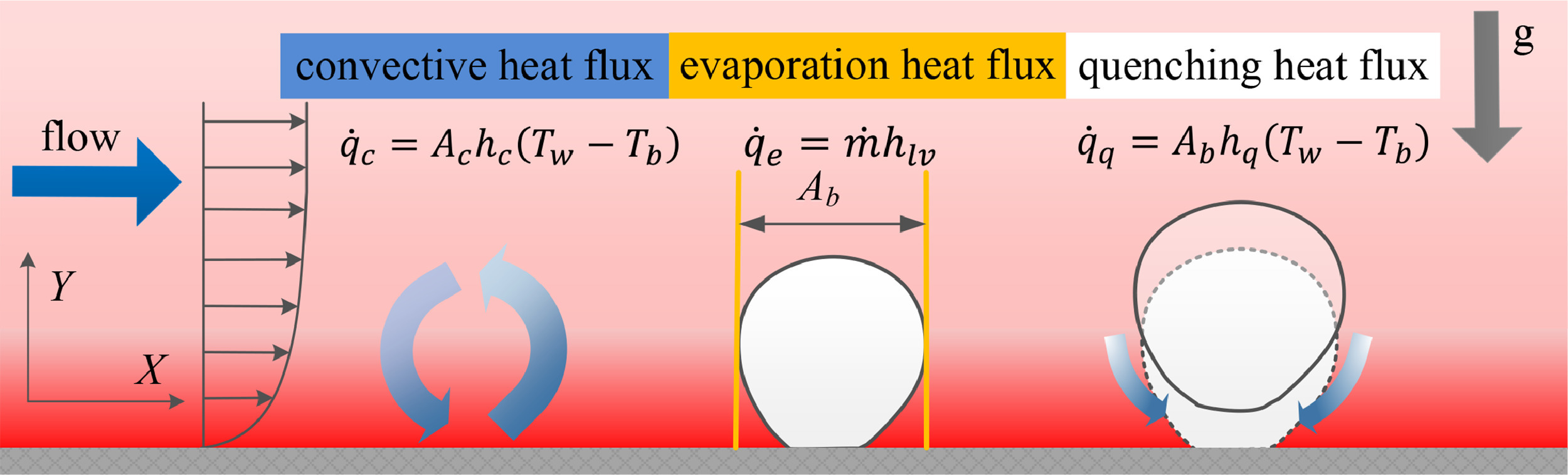
Figure 5 Depiction of the wall heat flux partitioning model for subcooled flow boiling from Zhou et al. [ZHG+21].#
The model is implemented in:
void Flux_parietal_Kurul_Podowski::set_param(Param& param)
The model implemented is decomposed as follows:
First, we have a Correction of single phase heat flux
\(\texttt{qpk}=\texttt{qpk}_{single\ phase}(1-A_{bub})\),
\(\texttt{da_qpk}=\texttt{da_qpk}_{single\ phase}(1-A_{bub})\),
\(\texttt{dp_qpk}=\texttt{dp_qpk}_{single\ phase}(1-A_{bub})\),
\(\texttt{dv_qpk}\texttt{=dv_qpk}_{single\ phase}(1-A_{bub})\),
\(\texttt{dTf_qpk}=\texttt{dT_f_qpk}_{single\ phase}(1-A_{bub})\),
\(\texttt{dTp_qpk}=\texttt{dTp_qpk}_{single\ phase}(1-A_{bub})\).
Then, we add the partitioned heat flux
\(\texttt{dTp_qpk} \pluseq -\texttt{qpk}_{single\ phase}(1-A_{bub})\frac{dA_{bub}}{dT_p}+\frac{dq_{quench}}{dT_p}\),
\(\texttt{qpk} \pluseq q_{quench}\),
\(\texttt{dTf_qpk} \pluseq \frac{dq_{quench}}{dT_l}\),
\(\texttt{qpi} \pluseq q_{evap}\),
\(\texttt{dTp_qpi} \pluseq \frac{dq_{evap}}{dT_p}\), with
Evaporation flux \(q_{evap}=f_{dep}\frac{\pi d_b^3}{6}\rho_gL_{vap}N_{sites}\)
Evaporation flux derivative regarding wall departure \(\frac{dq_{evap}}{dT_p} =(\frac{df_{dep}}{dT_p}\frac{\pi d_b^3}{6}N_{sites}+f_{dep}\frac{3\pi d^2}{6}\frac{dd_b}{dT_p}N_{sites}+f_{dep}\frac{\pi d_b^3}{6}\frac{dN_{sites}}{dT_p})\rho_g L_{vap}\).
Quenching flux \(q_{quench}=A_{bub}\sqrt{f_{dep}}\frac{2\lambda_l(T_p-T_l)}{\sqrt{\frac{\pi \lambda_l}{\rho_l Cp_l}}}\).
Quenching flux derivative regarding liquid temperature \(\frac{d q_{quench}}{d T_l} =A_{bub}\sqrt{f_{dep}}\frac{-2\lambda_l}{\sqrt{\frac{\pi \lambda_l}{\rho_l Cp_l}}}\).
Quenching flux derivative regarding wall temperature \(\frac{d q_{quench}}{d T_p} =\frac{d A_{bub}}{dT_p} \sqrt{f_{dep}}\frac{-2\lambda_l}{\sqrt{\frac{\pi \lambda_l}{\rho_l Cp_l}}}+A_{bub}\sqrt{f_{dep}}\frac{2\lambda_l}{\sqrt{\frac{\pi \lambda_l}{\rho_l Cp_l}}}-A_{bub}\frac{1}{2}\frac{df_{dep}}{dT_p}\frac{1}{\sqrt{f_{dep}}}\frac{2\lambda_l(T_p-T_l)}{\sqrt{\frac{\pi \lambda_l}{\rho_l Cp_l}}}\).
Number of evaporation sites \(N_{sites}=(210\times{}(T_p-T_{sat}))^{1.8}\).
Number of evaporation sites \(N_{sites}=(210\times{}(T_p-T_{sat}))^{1.8}\).
Number of evaporation sites derivative regarding wall temperature \(\frac{d N_{sites}}{dT_p} =210\times 1.8(210.(T_p-T_{sat}))^{0.8}\).
Wall bubble diameter \(d_b=0.0001(T_p-T_{sat})+0.0014\).
Wall bubble diameter derivative regrading wall temperature \(\frac{dd_b}{dT_p}=0.0001\).
Wall bubble total area \(A_{bub}=min(1.,\frac{\pi N_{sites}d_b^2}{4})\).
Wall bubble total area derivative regarding wall temperature \(\frac{dA_{bub}}{dT_p} =\frac{\pi d_b^2}{4}\frac{d N_{sites}}{dT_p} + \frac{\pi d_b N_{sites}}{2}\frac{d d_b}{dT_p}\), if \(A_{bubbles}\neq 1.\), \(0\), otherwise.
Departure frequency \(f_dep=\sqrt{\frac{4}{3}\frac{9.81(\rho_l-\rho_g)}{\rho_l}}d_b^{-0.5}\).
Departure frequency derivative regarding wall temperature \(\frac{d f_dep}{d T_p}=-0.5\frac{dd_b}{dT_p}d^{-1.5}\sqrt{\frac{4}{3}\frac{9.81(\rho_l-rho_g)}{\rho_l}}\)
Phase change#
The general expression of the phase change mass flux is:
It needs to be considered when there is a kinetic limit of gas for the phase change, for liquid metals, for example, but it does not apply to water.
The model is implemented in:
void Changement_phase_base::set_param(Param& param)
The available input parameters are:
    double D_h;           // Hydraulic diameter
    double p;             // Pressure
    const double *alpha;  // Void fraction
    const double *T;      // Temperature
    const double *lambda; // Thermal conductivity
    const double *mu;     // Viscosity
    const double *rho;    // Density
    const double *Cp;     // Calorific capacity
    const double *Lvap;   // Latent heat
    const double *Tsat;   //Phase change saturated temperature
The phase change mass flux operator must fill dT_G, da_G, dp_G tabs and there derivative so that:
\(\texttt{G}\) mass flux
\(\texttt{dT_G}\) mass flux derivative regarding temperature
\(\texttt{dp_G }\) mass flux derivative regarding pressure
\(\texttt{da_G}\) mass flux derivative regarding void fraction
Silver Simpson#
The model is also described in Silver and Simpson (1949, not found) and is implemented as:
void Changement_phase_Silver_Simpson::set_param(Param& param)
{
  param.ajouter("lambda_e", &lambda_ec[0]); multiplicative factor for evaporation
  param.ajouter("lambda_c", &lambda_ec[1]); //  multiplicative factor for condensation
  param.ajouter("alpha_min", &alpha_min); // minimal void fraction to activate phase change
  param.ajouter("M", &M, Param::REQUIRED); // molar mass of steam
}
Default values:
\(\texttt{lambda_ec[2]} = { 1, 1 }\),
\(\texttt{M} = -100.\),
\(\texttt{alpha_min} = 0.1\).
The model implemented is:
with
\(T_0 = 273.15\),
\(\texttt{var_ak}=\max(\alpha_g, \texttt{alpha_min})\),
\(\texttt{var_al}=\parent{\max\parent{\alpha_l,\texttt{alpha_min}}}^{1.5}\),
\(\texttt{var_a}=\texttt{var_ak} \times \texttt{var_al}\),
\(\texttt{var_T} = \frac{Psat(T_g)}{\sqrt{T_g + T_0}} - \frac{P}{\sqrt{T_l + T_0}}\),
\(\texttt{fac} = \lambda_{ec}[var_T < 0] \frac{4}{D_h}\sqrt{\frac{\texttt{M}}{2\texttt{M_{PI}}8.314}}\)